

Tropical cyclones (TCs) are characterized by spiraling winds that converge towards their center, lifting moisture to form clouds and precipitation.
These rainbands play a crucial role in global energy and water cycles and can cause significant flooding when TCs make landfall. Understanding how TC rainbands are organized is essential for improving forecasting systems and managing their impacts.
Previous studies have focused on temporal changes and used shape metrics for classification, but these approaches often lack consistency and objectivity. Recent advancements in autoencoders, particularly convolutional autoencoders (CAEs), offer a more robust solution.
CAEs excel in image clustering by learning local image structures, making them ideal for classifying complex TC rain patterns.In this study, we apply a CAE to classify nearly 12,000 rain images from North Atlantic TCs between 2000 and 2020.
Read More: Classifying Tropical Cyclone Rain Patterns with Convolutional Autoencoders
Convolutional Autoencoder (CAE) for Tropical Cyclone Rain Pattern Classification
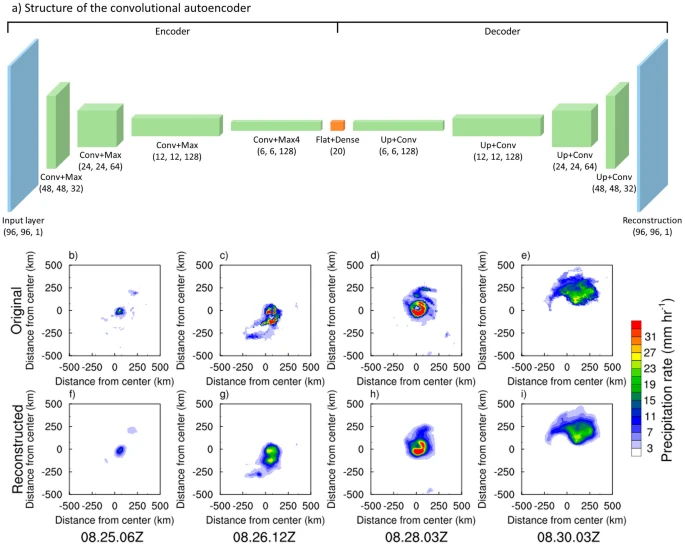
In this study, a convolutional autoencoder (CAE) is employed to classify tropical cyclone (TC) rain patterns. The CAE consists of an encoder that compresses the original image into low-dimensional features and a decoder that reconstructs the compressed features into an image resembling the original one.
The encoder is made up of an input layer followed by four consecutive convolution and max-pooling (Conv + Max) layers.
These layers progressively reduce the image’s width and height by half, transforming the original image size of 96×96 pixels into a compressed 6×6 pixels, while the depth of the feature maps increases, reaching 128.
This filtering and compression process is essential for the CAE to learn the relevant image features.
Following the encoder, the decoder mirrors the encoder’s structure with flattening and dense layers connected to four upsampling and convolution (Up + Conv) layers, ultimately producing an output layer with the same dimensions as the input.
The CAE learns the features of TC rain images by minimizing the difference between the original and reconstructed images. Figure 1(b−i) presents examples of original and reconstructed TC rain images from Hurricane Katrina (2005) at different times.
Despite minor differences, such as variations in the heavy rain areas (e.g., the red areas in Fig. 1c vs. Fig. 1g), the patterns between the original and reconstructed images are highly similar.
The pattern correlations between the original and reconstructed images range from 0.86 to 0.96, demonstrating the effectiveness of the training process.
To assess the performance of the CAE, we examine various metrics, including pattern correlation (PCOR), normalized standard deviation (NSTD), mean bias (MB), and root mean squared error (RMSE) between the original and reconstructed images.
The NSTD measures the ratio of the standard deviation of precipitation in the reconstructed image to that of the original image. Table 1 summarizes the mean and standard deviation of these metrics for 11,991 TC samples. The average PCOR is 0.892, which is significantly higher than results from simpler autoencoders.
The NSTD value close to 1 indicates that the variability in precipitation has been realistically reconstructed, and the low values of MB and RMSE further confirm the accuracy of the reconstruction.
The consistency of performance is demonstrated by the small standard deviations of these variables, further suggesting that the CAE successfully learned the features of TC rainfall patterns.
Classification of Tropical Cyclone (TC) Rain Patterns
The classification of tropical cyclone (TC) rain patterns is crucial for enhancing our understanding of the complex behavior and impacts of these storms.
Tropical cyclones are characterized by distinct rainband structures, which vary significantly depending on factors such as storm intensity, environmental conditions, and the underlying sea surface temperatures.
These rain patterns can range from tightly packed, intense precipitation near the storm’s center to broader, more diffuse rain areas on the outer edges.
Historically, researchers have used empirical metrics such as area, roundness, and dispersion to characterize TC rain shields.
However, these approaches can be limited by their reliance on hand-crafted features and may fail to capture the full complexity of TC rainfall structures.
Moreover, subjectivity in selecting shape descriptors can lead to inconsistencies in classification across different studies.
Properly classifying these patterns enables better predictions of rainfall distribution and intensity, which are vital for forecasting the storm’s potential to cause flooding and other weather-related hazards.
Traditional methods of classifying TC rain patterns typically rely on shape metrics and clustering techniques, yet these approaches can be subjective and prone to instability depending on the selected metrics.
Recent advancements in deep learning, particularly the use of convolutional autoencoders (CAEs), offer a promising approach to objectively classify TC rain patterns.
By compressing and reconstructing rain images, CAEs are capable of learning the underlying features of TC rainfall with high accuracy, providing more reliable classifications.
Such objective and robust classifications not only improve our ability to track and predict the behavior of tropical cyclones but also contribute to more accurate flood risk assessments and better preparedness for these extreme weather events.
Deep Learning-Based Classification of TC Rain Patterns Using Convolutional Autoencoders
Understanding the diverse rainfall structures of tropical cyclones (TCs) is vital for improving precipitation forecasting and advancing our knowledge of storm dynamics. However, objective systems for classifying TC rain patterns remain underdeveloped.
This study presents a novel approach using a Convolutional Autoencoder (CAE) to classify rain patterns in North Atlantic TCs.
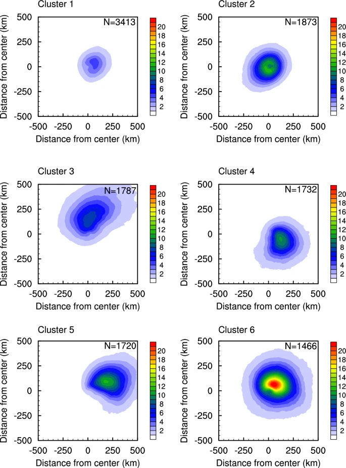
Through unsupervised learning, the CAE identified six optimal clusters, each reflecting distinct characteristics in terms of rainfall intensity, storm development stage, environmental conditions, and geographic location.
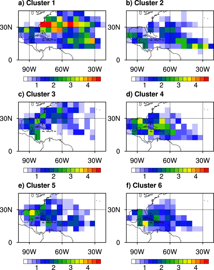
Cluster 1, the most frequent, featured weak, narrow precipitation, often corresponding to weakening TCs in mid-latitudes or early-stage systems in the Main Development Region (MDR).
In contrast, Cluster 2, though also forming in the MDR, displayed stronger rain in compact areas, typically in moist environments with low wind shear, representing more robust systems.
Cluster 3 exhibited the highest north–south asymmetry, the second-largest rain area, and was strongly influenced by vertical wind shear, appearing predominantly off the U.S. East Coast.
Clusters 4 and 5 revealed comma-shaped rain patterns with southeast and eastward asymmetries, common in the Gulf of Mexico and near the Antilles.
Finally, Cluster 6 represented mature TCs with the most intense and expansive rainfall, appearing mostly in the northwestern Caribbean, where deep tropical moisture is abundant.
This work is the first to apply deep learning for TC rain pattern classification, overcoming the subjectivity of earlier studies that relied on hand-selected shape metrics.
The CAE’s strength lies in its ability to extract features and distinguish structural differences objectively and efficiently, enabling the rapid classification of large datasets, including radar, reanalysis, and forecast products.
Looking forward, this framework will be extended to global ocean basins to explore both regional uniqueness and shared rainfall characteristics.
Additionally, long-term IMERG data will be used to assess temporal shifts in TC rain structures, potentially linked to increasing atmospheric moisture and climate-driven changes. This research opens new possibilities for enhancing our understanding and prediction of TC rainfall impacts worldwide.
Environmental Conditions Surrounding Tropical Cyclones
The moisture environment surrounding tropical cyclones (TCs) plays a critical role in modulating their structure and intensity.
This study defines the environmental moisture supply as the combined contribution of surface evaporation (EVAP) from warm ocean waters and vertically integrated moisture convergence (VIMC) within the troposphere.
These two components—EVAP and VIMC—represent the dominant mechanisms through which a TC accesses atmospheric moisture from its surrounding environment.In addition to moisture availability, vertical wind shear (VWS) was analyzed as a key environmental factor influencing TC development.
VWS refers to the vector difference in wind between the upper and lower troposphere—specifically between the 200 hPa and 850 hPa levels.
The shear was decomposed into north–south (VWS_NS) and east–west (VWS_EW) components, with positive values indicating southerly and westerly shear, respectively. The total vertical wind shear (VWS_TOT) was computed as the vector magnitude of these two components.
To ensure the focus remained on environmental influences rather than internal storm dynamics, the analysis excluded data within 200 km of the TC center, where the cyclone’s own circulation dominates. Environmental variables were averaged within an 800 km radius, providing a broader context.
Although an alternative approach using R17 (the radius of 17 m/s wind) was considered due to its relevance in representing the storm’s vortex scale, the results showed minimal difference from the fixed 200 km cutoff.
Therefore, for consistency and clarity, findings are reported using the standard 200 km exclusion radius.
Pre-processing of Tropical Cyclone Rainfall Data
Tropical cyclone (TC) rainfall images were extracted from the Integrated Multi-satellite Retrievals for GPM (IMERG) dataset by cropping a 96 × 96 pixel grid (approximately 1000 km × 1000 km) centered on the TC location.
Since these cropped images can include precipitation not directly associated with the TC, a filtering process was implemented to isolate the TC rain field:
- Rain polygons were identified, defined as contiguous pixel clusters with rainfall rates ≥ 1 mm h⁻¹.
- Polygons located more than 500 km from the TC center (minimum edge distance) were excluded to remove peripheral, unrelated precipitation.
This approach ensures focus on the primary rain structures of TCs—namely, the eyewall and spiral rainbands within a 500 km radius, which are most dynamically relevant. All rainfall values were normalized using the min–max method, rescaling rain rates to a range between 0 and 1.
TC center coordinates were obtained from the IBTrACS dataset, and rainfall images were acquired at 3-hour intervals. In total, 11,991 rainfall snapshots from 336 unique TCs (spanning 2000–2020) were compiled for analysis.
Shape Metrics for Rainfall Pattern Characterization
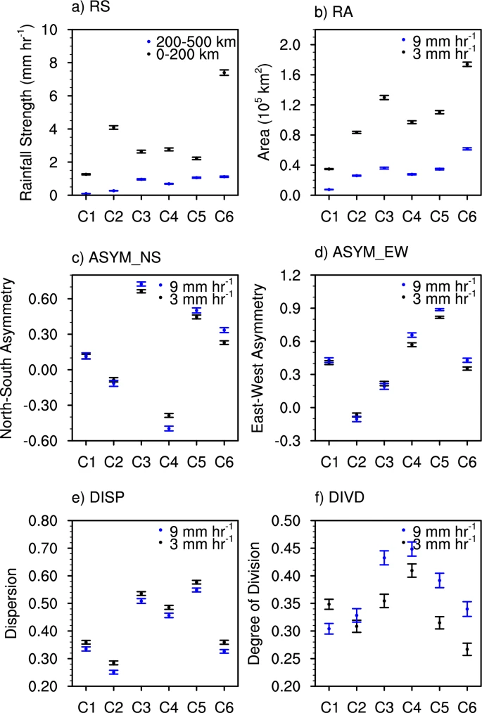
To quantify the morphology and intensity of TC rainfall, we evaluated rainfall strength and five shape-based metrics widely used in meteorological research.
- Rainfall Strength (RS) is defined as the average rain rate within a specific radial zone, including pixels with 0 mm h⁻¹ to capture overall precipitation magnitude. In this study, RS was computed separately for the 0–200 km (RS200) and 200–500 km (RS500) zones. The 200 km boundary effectively separates the near-core region from the outer rainbands, aligning with the average quadrant-mean R17 radius (~186 km).
- Rainfall Area (RA) represents the total surface area covered by the TC rain field, providing a measure of spatial extent.
- Rainfall Asymmetry was calculated in both north–south (ASYM_NS) and east–west (ASYM_EW) directions using: Equation (3)
ASYMNS=AN−ASAN+AS\text{ASYM}_{NS} = \frac{A_N – A_S}{A_N + A_S}ASYMNS=AN+ASAN−AS Equation (4)
ASYMEW=AE−AWAE+AW\text{ASYM}_{EW} = \frac{A_E – A_W}{A_E + A_W}ASYMEW=AE+AWAE−AW where AN,AS,AE,A_N, A_S, A_E,AN,AS,AE, and AWA_WAW are the respective areas of rainfall north, south, east, and west of the TC center. Positive values align with the hypothesized downshear displacement direction, often dictated by environmental wind shear. - Dispersion (DISP) quantifies how far the centroids of rain polygons are spread from the TC center. It is defined as: Equation (5)
DISP=∑(Ai⋅RiRsearch)\text{DISP} = \sum \left( \frac{A_i \cdot R_i}{R_{search}} \right)DISP=∑(RsearchAi⋅Ri) where AiA_iAi is the area and RiR_iRi is the centroid radius of the i-th rain polygon, and Rsearch=500R_{search} = 500Rsearch=500 km. Larger polygons are given higher weights in the calculation. - Degree of Division (DIVD) captures the fragmentation of the rain field and is defined by: Equation (6)
DIVD=1−(∑Ai2Atotal2)\text{DIVD} = 1 – \left( \frac{\sum A_i^2}{A_{total}^2} \right)DIVD=1−(Atotal2∑Ai2)
This metric reflects how the precipitation is broken into multiple discrete areas, with higher values indicating more fragmentation.
Clustering of Rainfall Patterns Using K-Means
To identify distinct spatial patterns in TC rainfall, we applied the k-means clustering algorithm to the compressed feature representations obtained from the convolutional autoencoder (CAE).
Specifically, the 96 × 96 images were passed through the CAE encoder, resulting in a 20-dimensional latent vector (see orange box in Fig. 1a). This dimensionality reduction enables more effective clustering, as applying k-means directly to high-dimensional image data would hinder classification performance.
K-means is an unsupervised learning algorithm that groups data based on intra-cluster similarity. The optimal number of clusters (k) was determined using the elbow method, which evaluates the total within-cluster sum of squares (WSS) as a function of k (Fig. S1).
While increasing k reduces WSS (i.e., enhances compactness), excessive clustering can lead to redundancy. The “elbow point,” where WSS reduction plateaus, typically indicates the most appropriate cluster count.
Based on this method, we determined that k = 6 provides the optimal clustering for Atlantic Basin TC rain patterns. We tested multiple values (k = 4 to 8) to evaluate stability and distinctiveness:
- Moving from k = 4 to k = 6, new clusters emerged that represented distinct rainfall asymmetries (e.g., west-heavy vs. east-heavy rain).
- At k ≥ 7, previously stable clusters began splitting into sub-clusters with minimal additional insight (e.g., cluster 3 dividing into two similar groups), suggesting diminishing returns.
Our conclusion that six clusters best represent the diversity in TC rainfall structures is further reinforced by environmental and statistical analyses, detailed below.
Statistical Validation of Cluster Distinctiveness
To assess whether the clusters represent statistically distinct rainfall distributions, we employed the Mann–Whitney U test, a non-parametric method for comparing two independent samples. The test evaluates whether two groups share the same median, with a significance threshold of α = 0.05.
- We performed 165 pairwise tests covering 11 rainfall distribution metrics across 15 cluster pairings (from the six-cluster solution).
- Additional tests compared storm intensity, moisture availability, and vertical wind shear (VWS) across clusters.
In cases where p < 0.05, the null hypothesis of identical medians was rejected, supporting the distinctiveness of the clusters. These results affirm that each cluster captures unique spatial and environmental characteristics of TC rainfall.
Frequently Asked Questions (FAQs)
How were the TC rain images generated?
TC rain images were derived by cropping the IMERG precipitation data into 96 × 96 pixel grids (~1000 km × 1000 km) centered on each TC. Only the rainfall directly associated with the TC was retained. This was done by identifying rain polygons (connected areas with rainfall ≥ 1 mm/h) and excluding those located more than 500 km from the TC center.
Why was a 500 km radius used to isolate TC-related rainfall?
This distance captures the primary rain structures of a TC, including the eyewall and spiral rainbands, while minimizing the influence of unrelated precipitation systems. It ensures that the focus remains on the core and immediate surroundings of the storm.
How was rainfall intensity normalized?
Rain rates in each image were normalized using the min–max method, scaling values to range from 0 to 1. This allowed consistent comparison across different storms and intensities.
What data source was used to determine the TC center?
The International Best Track Archive for Climate Stewardship (IBTrACS) dataset provided the official TC center positions, which were used for image alignment and metric calculations.
Why were 0–200 km and 200–500 km zones used to define rainfall strength?
These zones distinguish between the near-core region (typically encompassing the eyewall and inner rainbands) and the outer rainband region. The 200 km boundary closely aligns with average TC size characteristics found in previous research.
What is the purpose of the k-means clustering in this study?
K-means clustering was used to classify spatial patterns of TC rainfall. Rather than clustering raw images, the algorithm was applied to 20-dimensional feature vectors extracted from the encoder part of a Convolutional Autoencoder (CAE), which reduced dimensionality while preserving key spatial information.
Conclusion
This study presents a novel framework for classifying tropical cyclone (TC) rainfall structures by integrating physically interpretable shape metrics with advanced deep learning techniques. By focusing on the spatial distribution of rainfall within a 500 km radius of each storm and normalizing rain intensity using a min–max approach, we isolated the core TC-related precipitation features. Six key shape metrics—rainfall strength, area, asymmetry, dispersion, and division—provided a quantitative foundation for characterizing rain fields.